Using the same MLB run differential data that I have visualized before, I create a story which walks you through the data and insights I uncover. From a business perspective; story templates can be used to create an interactive presentation to walk an audience through some use-case scenarios. I sometimes use story to present data insights rather than collecting screenshots in PowerPoint. It allows the presenter to stay versatile and have the functionality to examine quick questions/different cuts of data brought up during the meeting.

Some cool things about story template:

• Collection of visualizations that discusses a data narrative
• Ability to walk your audience from data to insights to informed decisions
• You can add dashboards to each story point/page
• I find this option helpful to also show novice tableau users how to interact with Tableau dashboards
• You can make individual worksheets faster, by applying static filters and only using data elements needed for the specific view

Some limiations:

• Only one dashboard can be applied to a story page; whereas multiple dashboards/containers can be combined in a dashboard environment
• Dashboard environment may serve the same purpose with a neatly maintained group of tabs

What I think:

I like the functionality for high end data/tableau viewers; those that can connect the data sources and build on their own. In my experience, the dashboard functionality still is the go-to but the story mode can serve as a great compliment to those audience members that have solid foundations interacting with Tableau visualizations. While set in their way executives may be comfortable reviewing aggregated static snapshots; as the data culture in your workplace begins to evolve, the story mode can serve as the ad-hoc method to present.

---

Let’s discuss a real story I created:

Using MLB run differential data I was able to examine team performances since 1957. I selected some unique instances where some teams are identified as the highest/lowest run differential since 1957. I also looked at some other examples too. Using annotations we can call out or add some additional context to those examples.

Check out the view below:

When you start a new story; the above page/canvas will appear. Highlighted in yellow will be your available sheets/dashboards that you can work with. Circled in red is your canvas and in blue is your caption for the canvas, adding new story pages will add to the caption boxes. They will eventually serve as bookmarks to all your talking points or story pages.

Before you build, I like to conceptualize the story you are going to tell to you end-user. Remember, you are using story mode to unearth insights from a dashboard or set of worksheets to tell a story towards some conclusion. Let’s go back to my dataset looking at MLB run differential statistics.

What is the story I want to tell?

What insights can be derived?

Is Run Differential an important statistic to a team?

What instances support that or negate that?

A few things, I want to examine are how important the run differential statistic is to the offensive talent of a baseball team. Does it usually dictate world series contenders or playoff contenders. When compared to winning percentage, which measure is a better indicator of offensive talent. Looking at cohorts like team over the years divisions of teams at a time, we can immediately identify teams that have a history of offensive production (net runs) or years of bad baseball.

Below are some story snapshots I put together in the story I created:

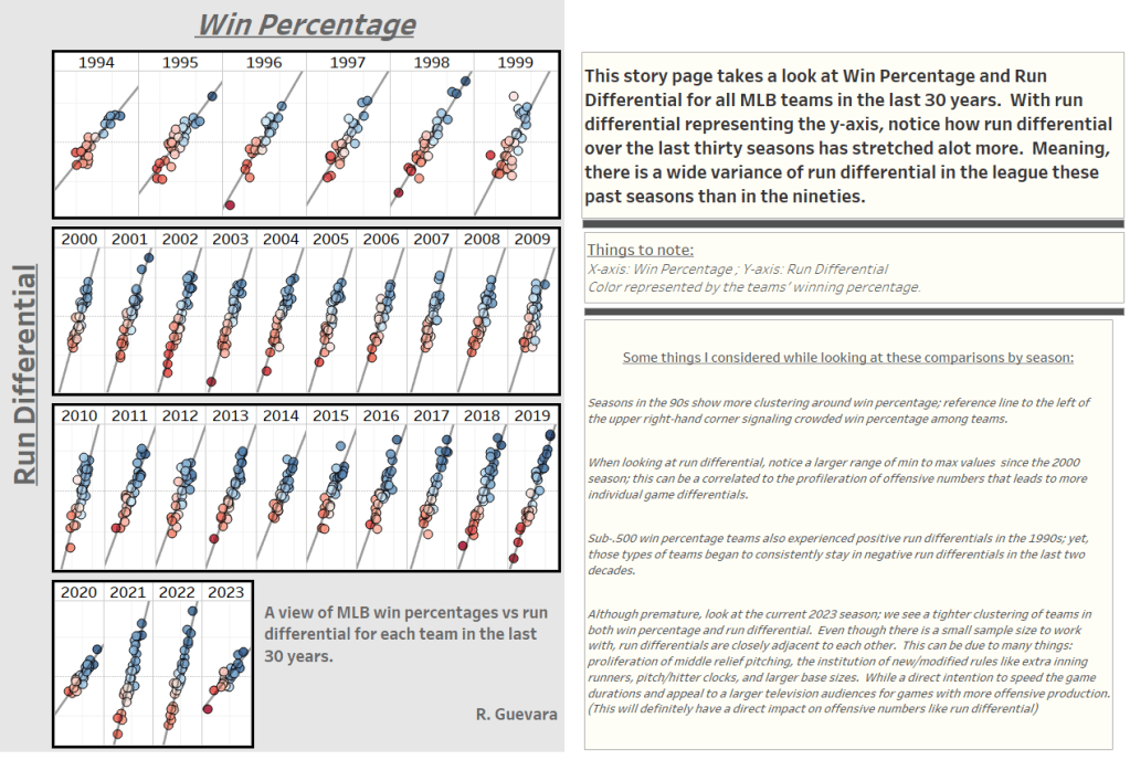
The above view shows run differential vs. win percentage for all teams in cohorts of seasons (for the last 30 years). Color palette is represented by teams’ winning percentage for that specific season.

Notice the movement of the reference line from 1994 to 2023 (as of May); this is a testament to how much run differential has evolved over the years. As more teams are producing more; the run differential disparity will increase resulting a more north-south display scatter plot marks in the cohort views.

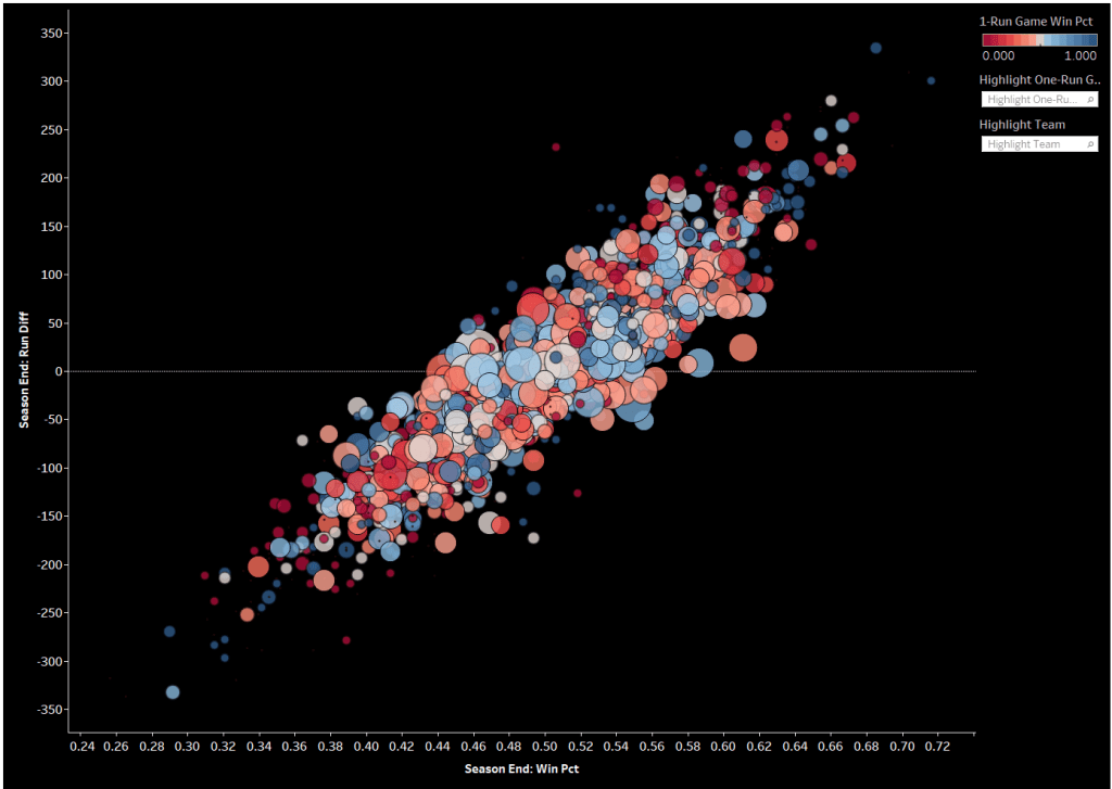
I like this view above, this looks at the same measures in the previous screenshot. Yet, all teams for each of their seasons are represented as a mark (circle) in the scatter plot. Color is represented as winning percentage in each teams’ one-run games. Size of the circle represents the number of one-run games for that respective teams season.

I personally like this view, the black background really makes the marks pop and some modification to the transparency adds depth to the number of marks in the scatter. You can use the highlight feature to view a team isolated or view marks with the same number of one-run games in the season. One thing I did notice, as you collect the one-run games, you begin to stay anchored toward the average run differential (closer to zero). Makes sense, as more teams lose or win by more than one run, the differential starts to sway away from that area.

I am also sure you have heard that saying in sports; any given day. Any team can have a great game or terrible game. This is baseball, they play 160+ games a season, so it only makes sense that teams that accumulate one-run games will win around .3 to .5 of those games (an average score). There are a few outliers to this; can you spot them while interacting with the dashboard?

I like the above views, it isolates three specific teams in their run differential performance. The third view that looks at run differential range; its unique to view this way because it clearly shows the consistent change in run differential. I took the season end run differential and peeled out the min range from end to its specific min/max run differential data point.

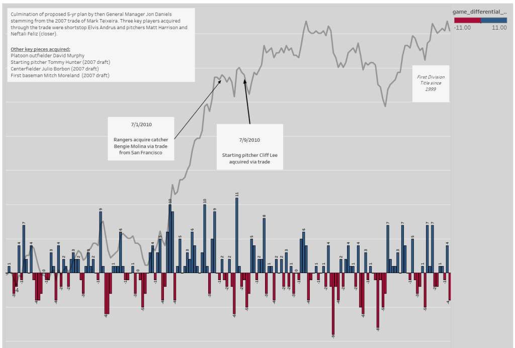
The last view I would like to show is a naturally biased choice. Yes, this is my team; as an avid Texas Rangers fan this specific team (2010 season) holds a special place in my sports heart.

The 2010 Texas Rangers ending the season with a run differential of 100; reaching a max run differential of 104 in August and only resulting in a negative run differential on three occasions throughout the whole season. I probably had the most annotations that I can confidently add because I vividly remember following this team and probably attending around 15+ games that season.

A few annotations that add substance to the 2010 run differential view:

• 7/1/2010: Bengie Molina (catcher) acquired
• 7/9/2010: Starting Pitcher Cliff Lee acquired via trade
• Cumulative result of the Mark Teixeira trade executed five years ago that brought a handful of key players that proved to be impactful in the 2010 season

Texas Rangers reached the World Series for the first time besting the New York Yankees in the American League Championship Series. Unfortunately, the Rangers lost to the San Francisco Giants in the World Series; I was actually there that game when the Giants clinched. It was hard to watch but so proud of my Rangers and what resulted to be a special season for the Texas boys.

Let’s wrap up

We took a created dashboard looking at MLB teams since 1957 and their respective run differential performances throughout the season. Using the Tableau story mode template, we identified specific instances of teams where run differential emerged as the worst/best in comparison to their other teams. We also examined run differential in comparison to win percentage to view the impact of offensive production vs. their respective win percentage. We also looked at the occurrence of one-run games that have the smallest weighted impact to run differential but the same consistent impact to a teams win percentage. Meaning a team can have a very high win percentage (accumulating one-run wins) while its run differential stays closer to zero. As teams collect blowout wins/losses their run differential results sways away from the zero line in a line chart.

Using story mode, we parsed out specific examples that really describe how run differential can vary for every team. We were also able to use annotations to point out specific areas/points in time to explain certain changes in the data. To learn more about story mode templates in Tableau check out the button below.

I hope you enjoyed this post and would love to hear any feedback you have for me.

Cheers,

Rafael